Histograms & Contrast Enhancement

A histogram is like a census for your image — instead of counting people by age, you’re counting pixels by brightness. This “population chart” reveals exposure problems that are invisible to the naked eye and enables powerful contrast enhancement techniques.

Computing Histograms with cv2.calcHist()

cv2.calcHist() counts how many pixels have each intensity value (0-255):

Python

import cv2
import numpy as np
import matplotlib.pyplot as plt

img = cv2.imread("photo.jpg", cv2.IMREAD_GRAYSCALE)

# Compute the histogram
# Parameters: [image], [channel], mask, [bins], [range]
hist = cv2.calcHist([img], [0], None, [256], [0, 256])

# Plot it
plt.figure(figsize=(8, 4))
plt.plot(hist, color='gray')
plt.fill_between(range(256), hist.flatten(), alpha=0.3, color='gray')
plt.xlabel("Pixel Intensity")
plt.ylabel("Number of Pixels")
plt.title("Image Histogram")
plt.xlim([0, 256])
plt.show()

Caution

The Bracket Trap: cv2.calcHist() expects the image wrapped in a list: [img], not img. Same for channels and other parameters. This is because it can compute histograms for multiple images and channels at once.

Color Histograms

For color images, compute separate histograms for each BGR channel:

Python

img_color = cv2.imread("photo.jpg")

colors = ('b', 'g', 'r')
plt.figure(figsize=(8, 4))

for i, color in enumerate(colors):
    hist = cv2.calcHist([img_color], [i], None, [256], [0, 256])
    plt.plot(hist, color=color, label=color.upper())

plt.legend()
plt.xlabel("Pixel Intensity")
plt.ylabel("Number of Pixels")
plt.xlim([0, 256])
plt.show()

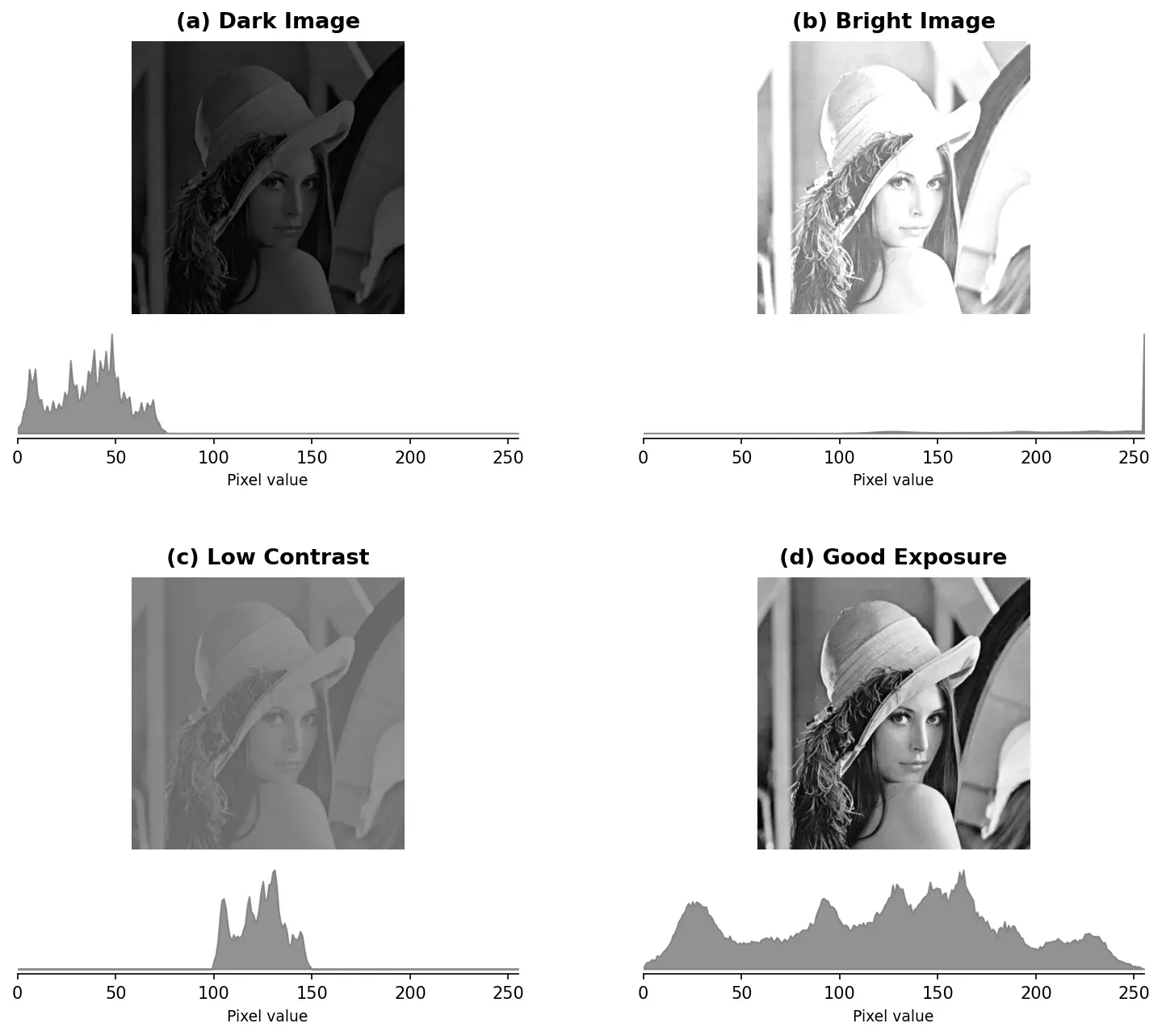
What Histograms Tell You

The shape of a histogram immediately reveals the image’s exposure quality:

Histogram Equalization

cv2.equalizeHist() redistributes pixel values so they spread evenly across the full range. It stretches the contrast by remapping intensities using the cumulative distribution function (CDF).

Python

# Input must be grayscale
equalized = cv2.equalizeHist(gray)

The result: dark images get brighter, faded images gain contrast, and the histogram becomes more uniform.

Caution

Never equalize BGR channels independently! If you apply equalizeHist() to each B, G, R channel separately, the color balance shifts dramatically (blue skies might turn green). Instead, convert to a color space that separates luminance from color, equalize only the luminance, then convert back:

Python

# WRONG — shifts colors
b, g, r = cv2.split(img)
b = cv2.equalizeHist(b)
g = cv2.equalizeHist(g)
r = cv2.equalizeHist(r)
bad = cv2.merge([b, g, r])

# CORRECT — equalize luminance only (via YUV)
yuv = cv2.cvtColor(img, cv2.COLOR_BGR2YUV)
yuv[:, :, 0] = cv2.equalizeHist(yuv[:, :, 0])
good = cv2.cvtColor(yuv, cv2.COLOR_YUV2BGR)

CLAHE — The Smart Equalizer

Global histogram equalization has a problem: it applies the same transformation everywhere. In an image with both dark and bright regions, equalizing globally can over-amplify noise in already-bright areas while still leaving dark areas underwhelming.

CLAHE (Contrast Limited Adaptive Histogram Equalization) solves this by:

1. Dividing the image into small tiles
2. Equalizing each tile independently
3. Limiting the contrast amplification (the “CL” in CLAHE) to prevent noise amplification
4. Blending tile boundaries smoothly

Python

# Create a CLAHE object
# clipLimit: contrast limiting factor (higher = more contrast, more noise)
# tileGridSize: number of tiles (8x8 means the image is divided into 64 regions)
clahe = cv2.createCLAHE(clipLimit=2.0, tileGridSize=(8, 8))

# Apply to a grayscale image
enhanced = clahe.apply(gray)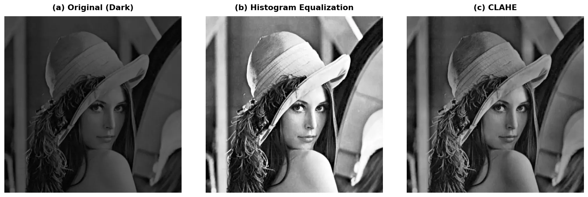

CLAHE Parameters

• clipLimit (default 40.0): Controls how much contrast is amplified. Lower values (1.0-3.0) give subtle enhancement. Higher values amplify more but risk reintroducing noise. Start with 2.0.
• tileGridSize (default (8, 8)): Controls how “local” the equalization is. Smaller tiles = more adaptive. Larger tiles = closer to global equalization.

Tip

CLAHE on LAB is a standard technique. For color images, convert to LAB, apply CLAHE to just the L (lightness) channel, then convert back. This enhances contrast without shifting colors — it’s widely used in face recognition, medical imaging, and photo enhancement.

Practical Example: Enhance an Underexposed Photo

1. Load the dark/underexposed image:

   Python

   import cv2
   
   img = cv2.imread("dark_photo.jpg")
   if img is None:
       raise FileNotFoundError("Could not load image!")

2. Convert to LAB color space:

   Python

   lab = cv2.cvtColor(img, cv2.COLOR_BGR2LAB)
   l_channel, a_channel, b_channel = cv2.split(lab)

3. Apply CLAHE to the L (lightness) channel:

   Python

   clahe = cv2.createCLAHE(clipLimit=2.0, tileGridSize=(8, 8))
   enhanced_l = clahe.apply(l_channel)

4. Merge channels and convert back to BGR:

   Python

   enhanced_lab = cv2.merge([enhanced_l, a_channel, b_channel])
   result = cv2.cvtColor(enhanced_lab, cv2.COLOR_LAB2BGR)

5. Display the result:

   Python

   cv2.imshow("Original (Dark)", img)
   cv2.imshow("CLAHE Enhanced", result)
   cv2.waitKey(0)
   cv2.destroyAllWindows()

Summary Checklist

• cv2.calcHist(): Pass [img] (list!), [channel], mask, [bins], [range]. Returns a 256×1 array of pixel counts.
• Reading histograms: Bunched left = dark, bunched right = bright, narrow peak = low contrast, spread = good exposure.
• cv2.equalizeHist(): Global contrast enhancement. Only works on single-channel (grayscale) images.
• Never equalize color channels independently — convert to YUV or LAB and equalize only the luminance channel.
• CLAHE: cv2.createCLAHE(clipLimit, tileGridSize). Local equalization that avoids over-amplifying noise. The go-to for real-world contrast enhancement.
• CLAHE on LAB: The standard recipe — convert to LAB, CLAHE the L channel, convert back. Works for any color image.