Drawing Basics

OpenCV provides a set of functions to draw geometric shapes directly onto images. Since images are just NumPy arrays, these functions modify the array in-place — they do not return a new image. Drawing is essential for visualizing computer vision results: bounding boxes around detected objects, keypoints on features, region overlays, and debug visualizations during development.

Every example on this page creates a blank canvas with np.zeros() so you can run them without any external images.

The Coordinate System

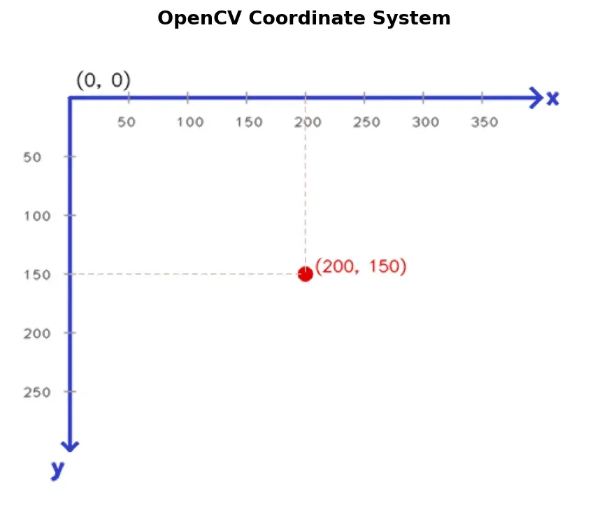
OpenCV uses a screen-style coordinate system. The origin (0, 0) is at the top-left corner of the image. The x-axis increases to the right and the y-axis increases downward. All drawing functions expect coordinates as (x, y) tuples — this is the opposite order from NumPy indexing, which uses (row, col).

Python

import cv2
import numpy as np

# Create a 400x500 black canvas (height=400, width=500, 3 channels)
canvas = np.zeros((400, 500, 3), dtype=np.uint8)

# Draw the x-axis (horizontal arrow)
cv2.arrowedLine(canvas, (10, 200), (490, 200), (255, 255, 255), 1, tipLength=0.03)
cv2.putText(canvas, "x", (470, 190), cv2.FONT_HERSHEY_SIMPLEX, 0.6, (255, 255, 255), 1)

# Draw the y-axis (vertical arrow)
cv2.arrowedLine(canvas, (250, 10), (250, 390), (255, 255, 255), 1, tipLength=0.03)
cv2.putText(canvas, "y", (260, 390), cv2.FONT_HERSHEY_SIMPLEX, 0.6, (255, 255, 255), 1)

# Mark the origin
cv2.circle(canvas, (250, 200), 4, (0, 0, 255), -1)
cv2.putText(canvas, "(0,0) origin", (260, 220), cv2.FONT_HERSHEY_SIMPLEX, 0.5, (0, 0, 255), 1)

cv2.imshow("Coordinate System", canvas)
cv2.waitKey(0)
cv2.destroyAllWindows()

Caution

Coordinates are (x, y) — horizontal first, vertical second. NumPy indexing is (row, col) which is (y, x). Mixing these up is one of the most common bugs when working with OpenCV drawing functions.

Color and Common Parameters

All drawing functions share a common set of parameters that control appearance.

Color

Color is specified as a BGR tuple (B, G, R) for 3-channel images. For single-channel grayscale images, pass a scalar integer. Some common colors in BGR:

• Red: (0, 0, 255)
• Green: (0, 255, 0)
• Blue: (255, 0, 0)
• White: (255, 255, 255)
• Yellow: (0, 255, 255)

Thickness

The thickness parameter controls the stroke width in pixels. A positive value draws an outline of that width. Passing -1 or cv2.FILLED fills the shape entirely.

Line Type

The lineType parameter controls how lines are rasterized:

• cv2.LINE_4 — 4-connected Bresenham line. Fastest but most jagged.
• cv2.LINE_8 — 8-connected Bresenham line. Default for all drawing functions.
• cv2.LINE_AA — Anti-aliased line using Gaussian filtering. Smoothest but slowest.

The shift parameter allows sub-pixel precision by treating coordinates as fixed-point numbers. This is advanced and rarely needed for typical drawing tasks.

Tip

Use cv2.LINE_AA for final visualizations and exported images — it produces noticeably smoother edges. Stick with the default cv2.LINE_8 for real-time or debug drawing where performance matters more than appearance.

Drawing Lines — cv2.line()

Python

cv2.line(img, pt1, pt2, color, thickness=1, lineType=cv2.LINE_8)

Draws a straight line from pt1 to pt2. Both points are (x, y) integer tuples.

Grid pattern

Python

import cv2
import numpy as np

canvas = np.zeros((400, 400, 3), dtype=np.uint8)

# Draw a grid with 50px spacing
for x in range(0, 401, 50):
    cv2.line(canvas, (x, 0), (x, 400), (40, 40, 40), 1)
for y in range(0, 401, 50):
    cv2.line(canvas, (0, y), (400, y), (40, 40, 40), 1)

# Draw thicker axis lines through the center
cv2.line(canvas, (200, 0), (200, 400), (0, 255, 0), 2)
cv2.line(canvas, (0, 200), (400, 200), (0, 255, 0), 2)

cv2.imshow("Grid", canvas)
cv2.waitKey(0)
cv2.destroyAllWindows()

Crosshair at center

Python

import cv2
import numpy as np

canvas = np.zeros((300, 300, 3), dtype=np.uint8)
cx, cy = 150, 150
size = 20

cv2.line(canvas, (cx - size, cy), (cx + size, cy), (0, 255, 255), 2, cv2.LINE_AA)
cv2.line(canvas, (cx, cy - size), (cx, cy + size), (0, 255, 255), 2, cv2.LINE_AA)

cv2.imshow("Crosshair", canvas)
cv2.waitKey(0)
cv2.destroyAllWindows()

Drawing Rectangles — cv2.rectangle()

Python

cv2.rectangle(img, pt1, pt2, color, thickness=1, lineType=cv2.LINE_8)

Draws a rectangle defined by its top-left corner pt1 and bottom-right corner pt2. You can also pass a tuple (x, y, w, h) as rec in the alternative form, but the two-point form is far more common.

Caution

pt1 and pt2 are the top-left and bottom-right corners of the rectangle — NOT center and size. If you have center and dimensions, compute the corners first: pt1 = (cx - w//2, cy - h//2) and pt2 = (cx + w//2, cy + h//2).

Outlined bounding box

Python

import cv2
import numpy as np

canvas = np.zeros((400, 400, 3), dtype=np.uint8)

# Draw an outlined rectangle (simulating a bounding box)
cv2.rectangle(canvas, (80, 60), (320, 340), (0, 255, 0), 2)

cv2.imshow("Bounding Box", canvas)
cv2.waitKey(0)
cv2.destroyAllWindows()

Filled semi-transparent rectangle

OpenCV does not support alpha blending directly, but you can achieve transparency by drawing on a copy and blending with cv2.addWeighted().

Python

import cv2
import numpy as np

canvas = np.zeros((400, 400, 3), dtype=np.uint8)

# Draw some background content
cv2.circle(canvas, (200, 200), 80, (255, 255, 255), 2)
cv2.putText(canvas, "Background", (120, 210), cv2.FONT_HERSHEY_SIMPLEX, 0.7, (255, 255, 255), 1)

# Create an overlay for the semi-transparent rectangle
overlay = canvas.copy()
cv2.rectangle(overlay, (50, 50), (350, 150), (255, 0, 0), cv2.FILLED)

# Blend: 60% original + 40% overlay
alpha = 0.4
cv2.addWeighted(overlay, alpha, canvas, 1 - alpha, 0, canvas)

cv2.imshow("Semi-Transparent Rectangle", canvas)
cv2.waitKey(0)
cv2.destroyAllWindows()

Drawing Circles — cv2.circle()

Python

cv2.circle(img, center, radius, color, thickness=1, lineType=cv2.LINE_8)

Draws a circle with the given center (x, y) and radius in pixels. Pass thickness=-1 to fill.

Concentric circles (bullseye)

Python

import cv2
import numpy as np

canvas = np.zeros((400, 400, 3), dtype=np.uint8)
center = (200, 200)
colors = [(0, 0, 255), (0, 165, 255), (0, 255, 255), (0, 255, 0), (255, 0, 0)]

for i, color in enumerate(colors):
    radius = 180 - i * 35
    cv2.circle(canvas, center, radius, color, 2, cv2.LINE_AA)

# Filled center dot
cv2.circle(canvas, center, 10, (255, 255, 255), -1, cv2.LINE_AA)

cv2.imshow("Bullseye", canvas)
cv2.waitKey(0)
cv2.destroyAllWindows()

Filled circles as dot markers

Python

import cv2
import numpy as np

canvas = np.zeros((300, 300, 3), dtype=np.uint8)

# Simulate detected keypoints
keypoints = [(50, 80), (150, 200), (250, 120), (100, 260), (220, 50)]

for pt in keypoints:
    cv2.circle(canvas, pt, 6, (0, 255, 0), -1, cv2.LINE_AA)     # filled dot
    cv2.circle(canvas, pt, 12, (0, 255, 0), 1, cv2.LINE_AA)      # outer ring

cv2.imshow("Keypoints", canvas)
cv2.waitKey(0)
cv2.destroyAllWindows()

Drawing Ellipses — cv2.ellipse()

Python

cv2.ellipse(img, center, axes, angle, startAngle, endAngle, color, thickness=1, lineType=cv2.LINE_8)

This function has several parameters:

• center — (x, y) center of the ellipse.
• axes — (major_half, minor_half) — half-lengths of the major and minor axes.
• angle — Rotation of the ellipse in degrees (clockwise).
• startAngle / endAngle — Angular range to draw, in degrees. Use 0 to 360 for a full ellipse.

Rotated ellipse

Python

import cv2
import numpy as np

canvas = np.zeros((400, 400, 3), dtype=np.uint8)

# Full ellipse rotated 30 degrees
cv2.ellipse(canvas, (200, 200), (150, 80), 30, 0, 360, (0, 255, 255), 2, cv2.LINE_AA)

# Same ellipse without rotation for comparison
cv2.ellipse(canvas, (200, 200), (150, 80), 0, 0, 360, (100, 100, 100), 1, cv2.LINE_AA)

cv2.imshow("Rotated Ellipse", canvas)
cv2.waitKey(0)
cv2.destroyAllWindows()

Arc and pie segment

You can draw partial ellipses by setting startAngle and endAngle to values other than 0 and 360. A filled partial ellipse creates a pie-chart-like wedge.

Python

import cv2
import numpy as np

canvas = np.zeros((400, 400, 3), dtype=np.uint8)

# Arc from 0 to 270 degrees (outline only)
cv2.ellipse(canvas, (150, 200), (100, 60), 0, 0, 270, (255, 0, 255), 2, cv2.LINE_AA)

# Filled pie segment from 0 to 270 degrees
cv2.ellipse(canvas, (300, 200), (80, 80), 0, 0, 270, (0, 200, 200), cv2.FILLED, cv2.LINE_AA)

cv2.imshow("Arc and Pie", canvas)
cv2.waitKey(0)
cv2.destroyAllWindows()

Note

Angles in cv2.ellipse() are measured clockwise from the positive x-axis (3 o’clock position). This follows the screen coordinate convention where y increases downward. A startAngle of 0 and endAngle of 90 draws the bottom-right quarter.

Drawing Polygons — cv2.polylines() and cv2.fillPoly()

Python

cv2.polylines(img, pts, isClosed, color, thickness=1, lineType=cv2.LINE_8)
cv2.fillPoly(img, pts, color, lineType=cv2.LINE_8)

Both functions accept pts as a list of arrays, where each array has shape (N, 1, 2) and dtype np.int32. The isClosed parameter in polylines determines whether the last point connects back to the first.

Caution

The pts arrays must be np.int32 with shape (N, 1, 2). If you have a plain list of points, convert it with: pts = np.array([[x1,y1],[x2,y2],...], dtype=np.int32).reshape((-1, 1, 2)). Forgetting the reshape or using the wrong dtype is a very common source of errors.

Triangle outline

Python

import cv2
import numpy as np

canvas = np.zeros((400, 400, 3), dtype=np.uint8)

triangle = np.array([[200, 50], [50, 350], [350, 350]], dtype=np.int32)
triangle = triangle.reshape((-1, 1, 2))

cv2.polylines(canvas, [triangle], isClosed=True, color=(0, 255, 0), thickness=2, lineType=cv2.LINE_AA)

cv2.imshow("Triangle", canvas)
cv2.waitKey(0)
cv2.destroyAllWindows()

Filled pentagon

Python

import cv2
import numpy as np

canvas = np.zeros((400, 400, 3), dtype=np.uint8)

# Regular pentagon centered at (200, 200)
angles = np.linspace(0, 2 * np.pi, 6)[:-1] - np.pi / 2  # start from top
radius = 120
cx, cy = 200, 200
pentagon = np.array([
    [int(cx + radius * np.cos(a)), int(cy + radius * np.sin(a))]
    for a in angles
], dtype=np.int32).reshape((-1, 1, 2))

cv2.fillPoly(canvas, [pentagon], (255, 100, 50))

cv2.imshow("Pentagon", canvas)
cv2.waitKey(0)
cv2.destroyAllWindows()

Multiple polygons at once

You can pass multiple arrays in the pts list to draw several polygons in a single call.

Python

import cv2
import numpy as np

canvas = np.zeros((400, 600, 3), dtype=np.uint8)

square = np.array([[50, 50], [200, 50], [200, 200], [50, 200]], dtype=np.int32).reshape((-1, 1, 2))

diamond = np.array([[400, 50], [500, 150], [400, 250], [300, 150]], dtype=np.int32).reshape((-1, 1, 2))

arrow = np.array([[250, 280], [350, 280], [350, 260], [420, 300],
                   [350, 340], [350, 320], [250, 320]], dtype=np.int32).reshape((-1, 1, 2))

# Draw all three outlines in one call
cv2.polylines(canvas, [square, diamond, arrow], isClosed=True,
              color=(0, 200, 255), thickness=2, lineType=cv2.LINE_AA)

cv2.imshow("Multiple Polygons", canvas)
cv2.waitKey(0)
cv2.destroyAllWindows()

Practical Example — Drawing Bounding Boxes with Labels

In object detection, the standard visualization pattern is to draw a colored rectangle around each detection and place a text label above it. The following example demonstrates this common workflow on a blank canvas.

Python

import cv2
import numpy as np

canvas = np.zeros((500, 700, 3), dtype=np.uint8)

# Simulated detections: (label, confidence, x1, y1, x2, y2, color)
detections = [
    ("person", 0.95, 50, 80, 220, 450, (0, 255, 0)),
    ("dog", 0.87, 260, 250, 450, 440, (255, 165, 0)),
    ("car", 0.73, 480, 100, 670, 320, (0, 0, 255)),
]

font = cv2.FONT_HERSHEY_SIMPLEX
font_scale = 0.6
font_thickness = 1

for label, conf, x1, y1, x2, y2, color in detections:
    # Draw bounding box
    cv2.rectangle(canvas, (x1, y1), (x2, y2), color, 2)

    # Prepare label text
    text = f"{label} {conf:.2f}"
    (text_w, text_h), baseline = cv2.getTextSize(text, font, font_scale, font_thickness)

    # Draw filled rectangle behind the text for readability
    cv2.rectangle(canvas, (x1, y1 - text_h - baseline - 4), (x1 + text_w + 4, y1), color, cv2.FILLED)

    # Draw label text in black on the colored background
    cv2.putText(canvas, text, (x1 + 2, y1 - baseline - 2), font, font_scale, (0, 0, 0), font_thickness, cv2.LINE_AA)

cv2.imshow("Object Detection Visualization", canvas)
cv2.waitKey(0)
cv2.destroyAllWindows()

This pattern scales to any number of detections. In a real pipeline you would replace the hardcoded detections list with output from a model — each item typically contains a class label, confidence score, and bounding box coordinates. The cv2.getTextSize() call ensures the label background always fits the text exactly regardless of font or string length.

Tip

When drawing on real camera frames at high speed, skip cv2.LINE_AA and use the default cv2.LINE_8 to keep drawing overhead minimal. Reserve anti-aliased drawing for saved images, screenshots, or low-FPS pipelines where visual quality matters.