Edge Detection & Gradients

Edges are where the action is. They mark boundaries between objects, transitions between colors, and outlines of shapes. Finding edges is often the last preprocessing step before “real” computer vision — contour detection, feature matching, and object recognition all start with edges.

What is an Edge?

An edge is a sharp change in pixel intensity. Mathematically, it’s where the gradient (first derivative) of the image is large.

Pixel row:     [10, 10, 10, 200, 200, 200]
                         ↑
                    EDGE HERE
           (intensity jumps from 10 to 200)

The gradient at each pixel tells you two things:

• Magnitude: How strong the edge is (big jump = strong edge)
• Direction: Which way the intensity changes (horizontal, vertical, diagonal)

$G = \sqrt{G_x^2 + G_y^2}$

Where $G_x$ is the gradient in the horizontal direction and $G_y$ is the vertical gradient.

Sobel Operator

The Sobel operator computes gradients by convolving the image with two 3×3 kernels — one for horizontal changes ($G_x$) and one for vertical changes ($G_y$):

Sobel X (vertical edges):     Sobel Y (horizontal edges):
   ┌─────────────┐                 ┌────────────┐
   │ -1   0   +1 │                 │ -1  -2  -1 │
   │ -2   0   +2 │                 │  0   0   0 │
   │ -1   0   +1 │                 │ +1  +2  +1 │
   └─────────────┘                 └────────────┘

Python

import cv2
import numpy as np

img = cv2.imread("photo.jpg", cv2.IMREAD_GRAYSCALE)

# Always blur first to reduce noise
blurred = cv2.GaussianBlur(img, (5, 5), 0)

# Compute gradients in X and Y directions
# Use CV_64F to capture negative gradients (dark-to-light transitions)
sobel_x = cv2.Sobel(blurred, cv2.CV_64F, 1, 0, ksize=3)
sobel_y = cv2.Sobel(blurred, cv2.CV_64F, 0, 1, ksize=3)

# Convert back to uint8 (take absolute value first)
abs_x = cv2.convertScaleAbs(sobel_x)
abs_y = cv2.convertScaleAbs(sobel_y)

# Combine X and Y gradients
combined = cv2.addWeighted(abs_x, 0.5, abs_y, 0.5, 0)

Caution

The uint8 Trap: If you use the default ddepth (uint8), negative gradients get clipped to 0. This means dark-to-light transitions become invisible — you lose half your edges! Always use cv2.CV_64F and then cv2.convertScaleAbs():

Python

# WRONG — loses negative gradients
sobel = cv2.Sobel(img, cv2.CV_8U, 1, 0)

# CORRECT — captures all gradients, then takes absolute value
sobel = cv2.Sobel(img, cv2.CV_64F, 1, 0)
sobel = cv2.convertScaleAbs(sobel)

Scharr Operator

For 3×3 kernels, the Scharr operator is more accurate than Sobel. It uses different kernel values that better approximate the true gradient:

Python

# Scharr in X direction (more accurate than Sobel for 3x3)
scharr_x = cv2.Scharr(blurred, cv2.CV_64F, 1, 0)
scharr_x = cv2.convertScaleAbs(scharr_x)

Use Scharr when you’re using a 3×3 kernel and need maximum accuracy. For larger kernels (5×5, 7×7), Sobel is the better choice.

Laplacian

The Laplacian computes the second derivative of the image, detecting edges in all directions simultaneously. Unlike Sobel (which gives you separate X and Y), Laplacian outputs a single edge map.

$\Delta I = \frac{\partial^2 I}{\partial x^2} + \frac{\partial^2 I}{\partial y^2}$

Python

laplacian = cv2.Laplacian(blurred, cv2.CV_64F)
laplacian = cv2.convertScaleAbs(laplacian)

The trade-off: Laplacian is more sensitive to noise than Sobel because second derivatives amplify high-frequency noise. Always blur before using it.

Canny Edge Detection

Canny is the gold standard of edge detection. Developed by John Canny in 1986, it’s a multi-stage algorithm that produces clean, thin, well-connected edges. Most edge detection tasks should start here.

1. Gaussian Blur: Smooths noise (Canny does this internally, but pre-blurring often helps).

2. Gradient Computation: Calculates intensity gradients using Sobel (internally).

3. Non-Maximum Suppression: Thins the edges to 1-pixel width by keeping only the local maxima in the gradient direction.

4. Hysteresis Thresholding: Uses two thresholds to classify edge pixels:

   • Gradient > threshold2 (high) → Strong edge (definitely an edge)
   • Gradient < threshold1 (low) → Not an edge (discard)
   • In between → Weak edge (kept only if connected to a strong edge)

Python

# threshold1 = low threshold, threshold2 = high threshold
edges = cv2.Canny(blurred, threshold1=50, threshold2=150)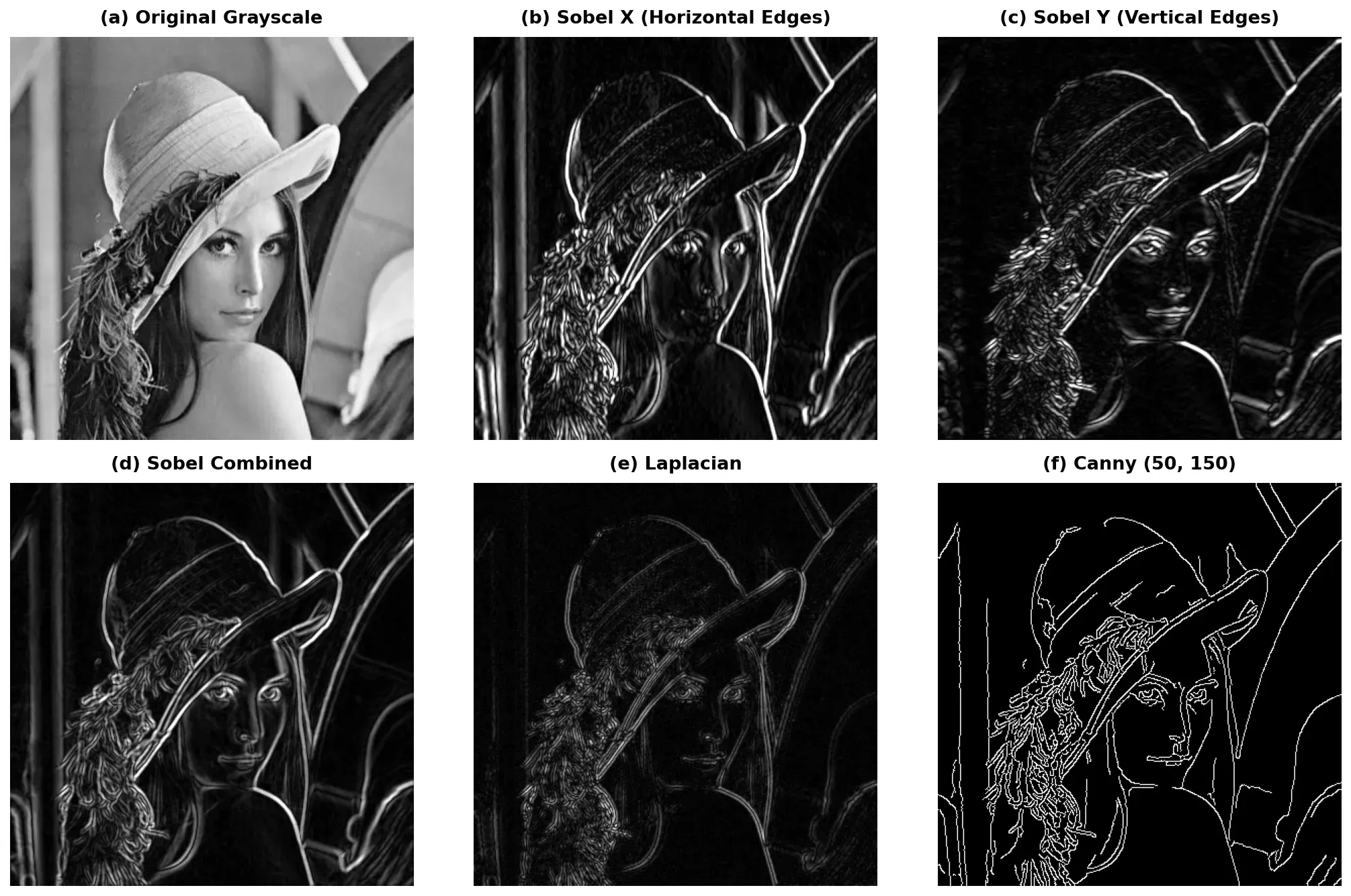

Choosing Canny Thresholds

The two thresholds control how sensitive Canny is:

• Low threshold1, low threshold2: Detects more edges (including noise)
• High threshold1, high threshold2: Detects only strong, obvious edges
• Common ratio: threshold1 = 0.5 * threshold2 works well as a starting point

Tip

A popular heuristic: Compute the median pixel intensity and use it to set thresholds:

Python

median = np.median(blurred)
lower = int(max(0, 0.7 * median))
upper = int(min(255, 1.3 * median))
edges = cv2.Canny(blurred, lower, upper)

Tip

Always blur before Canny. Even though Canny includes its own internal Gaussian blur, applying cv2.GaussianBlur() first gives you more control and usually produces cleaner results.

Choosing the Right Detector

Detector	Strengths	Weaknesses	Best For
Sobel	Fast, directional (X/Y separately)	Thick edges, needs combining	When you need gradient direction info
Scharr	More accurate than Sobel (3×3 only)	Same thickness issue as Sobel	Precision gradient calculation
Laplacian	Omnidirectional, single output	Very noise-sensitive	Quick edge overview, Blob detection
Canny	Clean, thin, connected edges	Two thresholds to tune	General-purpose edge detection

Tip

When in doubt, use Canny. It handles most edge detection scenarios well. Drop to Sobel when you need directional gradient information (e.g., for feature descriptors).

Practical Example: Full Edge Detection Pipeline

Python

import cv2
import numpy as np

# 1. Load the image
img = cv2.imread("photo.jpg")
if img is None:
    raise FileNotFoundError("Could not load image!")

# 2. Convert to grayscale
gray = cv2.cvtColor(img, cv2.COLOR_BGR2GRAY)

# 3. Blur to reduce noise
blurred = cv2.GaussianBlur(gray, (5, 5), 0)

# 4. Apply Canny edge detection
# Use the median heuristic for automatic threshold selection
median = np.median(blurred)
lower = int(max(0, 0.7 * median))
upper = int(min(255, 1.3 * median))
edges = cv2.Canny(blurred, lower, upper)

# 5. Display results
cv2.imshow("Original", img)
cv2.imshow("Edges (Canny)", edges)
cv2.waitKey(0)
cv2.destroyAllWindows()

Summary Checklist

• Image gradients: Rate of change in pixel intensity. Magnitude tells edge strength, direction tells edge orientation.
• cv2.Sobel(): Use cv2.CV_64F for ddepth, then cv2.convertScaleAbs(). Combine X and Y with cv2.addWeighted().
• cv2.Scharr(): More accurate than Sobel for 3×3 kernels. Same usage pattern.
• cv2.Laplacian(): Second derivative, omnidirectional. More noise-sensitive — always blur first.
• cv2.Canny(): The gold standard. Two thresholds control sensitivity. A good starting ratio is low = 0.5 * high.
• Always blur first: Noise creates false edges. GaussianBlur(img, (5,5), 0) before any edge detector.