Color Space Conversions

In the Fundamentals section, you learned what color spaces are — BGR, HSV, Grayscale, and YUV. Now it’s time to use them as preprocessing tools.

Color space conversion is often the very first step in any computer vision pipeline. Why? Because choosing the right color space makes downstream tasks (like detecting objects, segmenting regions, or enhancing contrast) dramatically easier.

The cv2.cvtColor() Toolkit

You’ve already seen cv2.cvtColor() for basic conversions. Here’s the complete reference for the conversions you’ll use most:

Conversion Code	From → To	When to Use
cv2.COLOR_BGR2GRAY	BGR → Grayscale	Edge detection, thresholding, most preprocessing
cv2.COLOR_BGR2HSV	BGR → HSV	Color-based object detection and filtering
cv2.COLOR_BGR2LAB	BGR → LAB	Contrast enhancement (CLAHE), perceptual comparisons
cv2.COLOR_BGR2RGB	BGR → RGB	Displaying with Matplotlib or saving for web
cv2.COLOR_GRAY2BGR	Grayscale → BGR	Adding color annotations to a grayscale result

Python

import cv2

img = cv2.imread("photo.jpg")
if img is None:
    raise FileNotFoundError("Could not load image. Check your path!")

# Convert to different color spaces
gray = cv2.cvtColor(img, cv2.COLOR_BGR2GRAY)
hsv = cv2.cvtColor(img, cv2.COLOR_BGR2HSV)
lab = cv2.cvtColor(img, cv2.COLOR_BGR2LAB)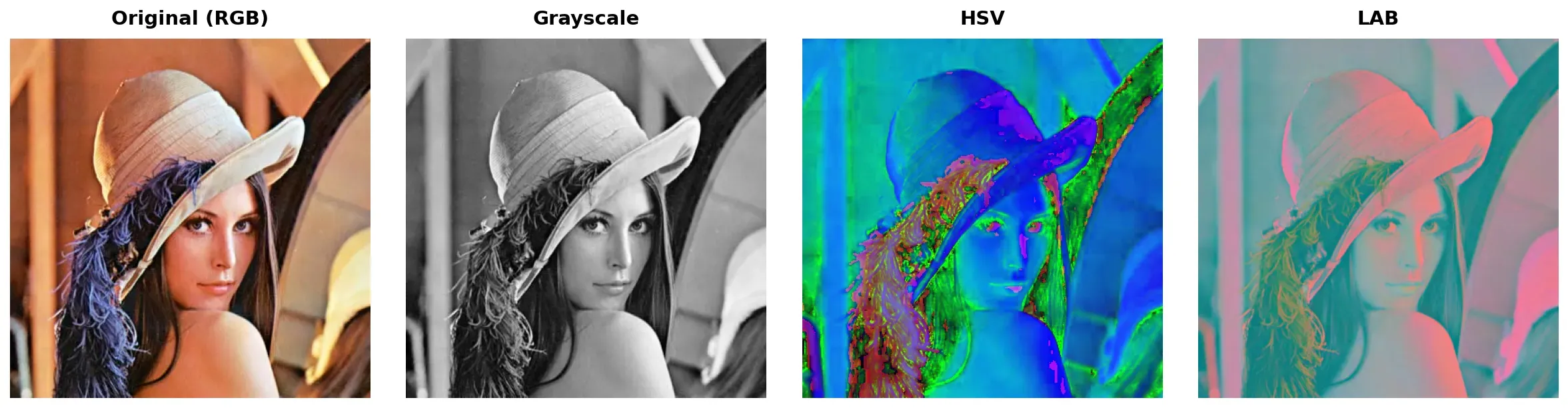

The LAB Color Space

You already know BGR, HSV, and Grayscale from Fundamentals. The one that didn’t get its spotlight is LAB (also written as L*a*b*), and it’s secretly one of the most useful color spaces for preprocessing.

LAB separates an image into three channels:

• L (Lightness): Pure brightness, from 0 (black) to 255 (white). Think of it as a “better grayscale.”
• a: Color range from Green (low values) to Red/Magenta (high values).
• b: Color range from Blue (low values) to Yellow (high values).

Why is this useful? LAB is perceptually uniform — a change of 10 units in LAB looks like the same amount of change to the human eye, no matter where you are on the scale. BGR and RGB don’t have this property (a jump from 100→110 in Red looks different than 200→210).

This makes LAB ideal for:

• Contrast enhancement: Apply CLAHE to just the L channel (we’ll cover this in the Histograms page).
• Color difference measurement: Comparing how “similar” two colors look to a human.
• Lighting-invariant operations: The L channel captures all the lighting; a and b capture pure color.

Python

# Convert to LAB
lab = cv2.cvtColor(img, cv2.COLOR_BGR2LAB)

# Split into channels
l_channel, a_channel, b_channel = cv2.split(lab)

# The L channel is a high-quality grayscale representation
# The a and b channels contain pure color information

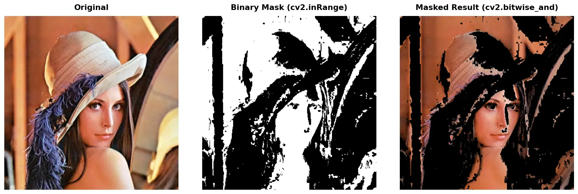
Color Filtering with cv2.inRange()

This is where color spaces become truly powerful as a preprocessing tool. cv2.inRange() lets you create a binary mask that isolates pixels within a specific color range — essentially saying “show me only the blue pixels” or “find everything that’s green.”

The workflow is always the same:

1. Convert to HSV — because HSV separates color (Hue) from lighting (Value), making your filter robust to shadows and brightness changes.

   Python

   import cv2
   import numpy as np
   
   img = cv2.imread("photo.jpg")
   hsv = cv2.cvtColor(img, cv2.COLOR_BGR2HSV)

2. Define your color range — pick lower and upper bounds for Hue, Saturation, and Value.

   Python

   # Example: Detect green objects
   # Hue: 35-85 (green range in OpenCV's 0-179 scale)
   # Saturation: 50-255 (ignore very faded pixels)
   # Value: 50-255 (ignore very dark pixels)
   lower_green = np.array([35, 50, 50])
   upper_green = np.array([85, 255, 255])

3. Create the mask — cv2.inRange() returns a binary image where white pixels are “in range” and black pixels are “out of range.”

   Python

   mask = cv2.inRange(hsv, lower_green, upper_green)
   # mask is a single-channel image: 255 where green, 0 elsewhere

4. Apply the mask — use cv2.bitwise_and() to keep only the pixels that passed the filter.

   Python

   result = cv2.bitwise_and(img, img, mask=mask)
   # result shows only the green parts of the original image

Common HSV Ranges

Here’s a cheat sheet for detecting common colors in OpenCV’s HSV scale (Hue: 0-179, Saturation: 0-255, Value: 0-255):

Color	Hue Low	Hue High	Notes
Red	0-10 and 170-179	—	Red wraps around! Need two masks.
Orange	10	25
Yellow	25	35
Green	35	85
Blue	85	130
Purple	130	170

Caution

The Red Wrap-Around Trap: In OpenCV’s HSV, Hue goes from 0 to 179. Red sits at both ends of this range (around 0-10 and 170-179). To detect red, you need two separate masks combined with cv2.bitwise_or():

Python

# Red detection requires two ranges
lower_red1 = np.array([0, 50, 50])
upper_red1 = np.array([10, 255, 255])
lower_red2 = np.array([170, 50, 50])
upper_red2 = np.array([10, 255, 255])

mask1 = cv2.inRange(hsv, lower_red1, upper_red1)
mask2 = cv2.inRange(hsv, lower_red2, upper_red2)
mask = cv2.bitwise_or(mask1, mask2)

Tip

Finding the right HSV range: Don’t guess! Load your target image, convert to HSV, and use print(hsv[y, x]) to read the HSV values of pixels you want to detect. Then build your range around those values with some tolerance (±10 for Hue is a good starting point).

Practical Example: Isolating a Colored Object

Here’s a complete pipeline that detects and isolates a blue object from a scene:

Python

import cv2
import numpy as np

# 1. Load the image
img = cv2.imread("scene.jpg")
if img is None:
    raise FileNotFoundError("Could not load image!")

# 2. Convert to HSV
hsv = cv2.cvtColor(img, cv2.COLOR_BGR2HSV)

# 3. Define blue range
lower_blue = np.array([85, 50, 50])
upper_blue = np.array([130, 255, 255])

# 4. Create binary mask
mask = cv2.inRange(hsv, lower_blue, upper_blue)

# 5. Optional: Clean up the mask with morphology
# (We'll cover this in detail in the Morphological Operations page)
kernel = np.ones((5, 5), np.uint8)
mask = cv2.morphologyEx(mask, cv2.MORPH_OPEN, kernel)
mask = cv2.morphologyEx(mask, cv2.MORPH_CLOSE, kernel)

# 6. Apply the mask to the original image
result = cv2.bitwise_and(img, img, mask=mask)

# 7. Display
cv2.imshow("Original", img)
cv2.imshow("Mask", mask)
cv2.imshow("Blue Objects Only", result)
cv2.waitKey(0)
cv2.destroyAllWindows()

Summary Checklist

• cv2.cvtColor(): Your gateway to all color space conversions. Know the major flags (BGR2GRAY, BGR2HSV, BGR2LAB, BGR2RGB).
• LAB color space: Use the L channel for contrast enhancement and perceptually uniform color comparisons.
• cv2.inRange(): Creates binary masks from HSV ranges. Always convert to HSV first for robust color filtering.
• Red wrap-around: Red hue spans both ends of the 0-179 range — combine two masks with cv2.bitwise_or().
• Mask application: Use cv2.bitwise_and(img, img, mask=mask) to apply a binary mask to an image.