Digital Images

To a computer, an image isn’t a photograph or a painting—it’s just a grid of numbers.

Understanding this numeric structure is the secret weapon of computer vision. Once you stop seeing “pictures” and start seeing “matrices,” operations like edge detection, color filtering, and object recognition become simply math problems.

The Pixel Grid

Imagine zooming into a photo until it turns into a blocky mosaic. Each of those blocks is a pixel (Picture Element), the fundamental atom of a digital image.

Coordinates: In OpenCV, we address pixels by (y, x) or (row, col). This is slightly counter-intuitive if you’re used to Cartesian (x, y) coordinates, but standard for matrices.
Resolution: Simply the dimensions of the grid. A 1920x1080 image is a grid 1080 rows tall and 1920 columns wide.

Under the Hood: It’s Just a Matrix

When you load an image in OpenCV, you aren’t getting a special “Image Object”—you’re getting a NumPy array.

This is one of OpenCV’s most powerful design choices. By using standard NumPy arrays, OpenCV images are compatible with the entire Python scientific ecosystem (like Matplotlib, Scikit-learn, and Pandas) right out of the box. You don’t need special converters; if you know how to work with data lists in Python, you already know how to edit images.

Grayscale: A 2D Sheet

A black-and-white (grayscale) image is the simplest form. It’s a 2D matrix (think of an Excel sheet) where each cell represents a single pixel’s intensity.

0 = Pure Black (No light)
255 = Pure White (Maximum light)
128 = Middle Gray

Computer vision algorithms often convert color images to grayscale first. Why? Because for tasks like detecting edges or reading text, you only care about light intensity shapes, not color. Dropping color reduces the data by 66%, making your code run significantly faster.

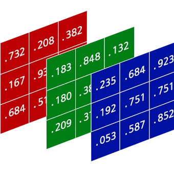
Image Matrix (8-bit grayscale), 3x3 pixels:
┌─────────────────┐
│   0   128   255 │  <- Row 0 (Black -> Gray -> White)
│ 255   128     0 │  <- Row 1 (White -> Gray -> Black)
│  50    50    50 │  <- Row 2 (Dark Gray line)
└─────────────────┘

Color: A 3D Stack

Color images add a third dimension. Instead of a single sheet of numbers, imagine three sheets stacked on top of each other. Each sheet represents a color channel: typically Blue, Green, and Red.

So, a single pixel isn’t just one number—it’s a vector of three numbers (B, G, R).

Pure Blue Pixel: [255, 0, 0] (Max Blue, No Green, No Red)
Pure Red Pixel: [0, 0, 255] (No Blue, No Green, Max Red)
White Pixel: [255, 255, 255] (Max of all colors)
Black Pixel: [0, 0, 0] (No light at all)

This structure (Height, Width, Channels) is why you’ll see shapes like (1080, 1920, 3).

Visualizing an image as a stack of three matrices

Code: Seeing the Matrix

Here is how this looks in actual Python code. Notice that “loading an image” is really just “loading a matrix from a file.”

import cv2
import numpy as np

# Load an image
img = cv2.imread('photo.jpg')

# 1. CHECK THE SHAPE
# .shape gives (Rows/Height, Columns/Width, Channels)
# If it returns (500, 500), it's grayscale (no channels dimension).
# If it returns (500, 500, 3), it's a color image.
print(f"Shape: {img.shape}")

# 2. READ A PIXEL
# Let's look at the pixel at Row 50, Column 100
px = img[50, 100]
print(f"Pixel value at (50, 100): {px}")
# Output: [240  50  50]  -> Roughly equivalent to Blue=240, Green=50, Red=50

# 3. MODIFY A PIXEL
# Change that pixel to pure Blue
img[50, 100] = [255, 0, 0] # [Blue, Green, Red]

Creating Images from Scratch

Since images are just arrays, we don’t need to load a file to have an image. We can create one mathematically using np.zeros() (which creates a matrix filled with 0s).

Why 0s? Because 0 is black. So np.zeros() effectively creates a black canvas.

# 1. Create a black canvas
# Dimensions: 480px tall, 640px wide, 3 channels (Color)
# dtype=np.uint8: CRITICAL! Images expect 8-bit integers (0-255).
# If you use floats, OpenCV might get confused.
canvas = np.zeros((480, 640, 3), dtype=np.uint8)

# 2. Draw a Blue line across the middle
# Set Row 240, All Columns (:), Channel 0 (Blue) to 255
canvas[240, :, 0] = 255

Color Depth (Bit Depth)

You’ll noticed we keep mentioning “0 to 255.” Why that specific range?

It comes down to memory efficiency. A standard image uses 8 bits (1 byte) to store each color value.

2^8 = 256 \text{ possibilities}

8-bit (uint8): The standard. 0-255 per channel. This gives us 16.7 million colors ( $256 \times 256 \times 256$ ), which is more than the human eye can distinguish.
16-bit / 32-bit (float): Sometimes 256 steps isn’t enough. For example, in Medical Imaging (X-Rays) or HDR Photography, you might need to distinguish between “dark gray” and “slightly lighter dark gray” with extreme precision. In those cases, we use 16-bit integers ( $0-65,535$ ) or 32-bit floating point numbers ( $0.0-1.0$ ).

Common Formats

You’ll encounter different wrappers for this data.

JPEG

The Photographer. Great for compressing real-world photos. It “throws away” invisible details to save space (lossy).

PNG

The Artist. Preserves every single pixel value exactly (lossless). Supports transparency. Great for screenshots and diagrams.

TIFF

The Archivist. Heavy, professional, often uncompressed. Used when quality matters more than disk space.

WebP

The Modernist. A newer format that often beats JPEG and PNG at their own game. Efficient for web.

Why This Matters

Understanding this structure explains why:

OpenCV is fast: It uses NumPy’s highly optimized array operations underneath.
Coordinates differ: Math matrices use (Row, Col) vs Cartesian (x, y).
Color spaces exist: Switching from BGR to Grayscale is just mathematically combining the 3 channels into 1.

Now that you know the matrix, you’re ready to start manipulating it.